Brillouin and Langevin functions

1 Brillouin Function
2 Langevin Function
3 High Temperature Limit
4 High Field Limit
5 References

Brillouin Function

The Brillouin function^[1]^[2] is a special function defined by the following equation:

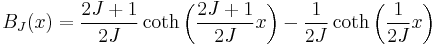
$B_J(x) = \frac{2J %2B 1}{2J} \coth \left ( \frac{2J %2B 1}{2J} x \right ) - \frac{1}{2J} \coth \left ( \frac{1}{2J} x \right )$

The function is usually applied (see below) in the context where x is a real variable and J is a positive integer or half-integer. In this case, the function varies from -1 to 1, approaching +1 as $x \to %2B\infty$ and -1 as $x \to -\infty$ .

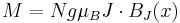
The function is best known for arising in the calculation of the magnetization of an ideal paramagnet. In particular, it describes the dependency of the magnetization $M$ on the applied magnetic field $B$ and the total angular momentum quantum number J of the microscopic magnetic moments of the material. The magnetization is given by:^[1]

$M = N g \mu_B J \cdot B_J(x)$

where

$N$ is the number of atoms per unit volume,
$g$ the g-factor,
$\mu_B$ the Bohr magneton,
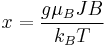
$x$ is the ratio of the Zeeman energy of the magnetic moment in the external field to the thermal energy $k_B T$ :

$x = \frac{g \mu_B J B}{k_B T}$

$k_B$ is the Boltzmann constant and $T$ the temperature.

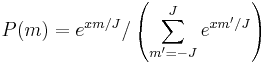
Click "show" to see a derivation of this law:

A derivation of this law describing the magnetization of an ideal paramagnet is as follows.^[1] Let z be the direction of the magnetic field. The z-component of the angular momentum of each magnetic moment (a.k.a. the azimuthal quantum number) can take on one of the 2J+1 possible values -J,-J+1,...,+J. Each of these has a different energy, due to the external field B: The energy associated with quantum number m is

$E_m = -mg \mu_B B = -k_BTxm/J$

(where g is the g-factor, μ_B is the Bohr magneton, and x is as defined in the text above). The relative probability of each of these is given by the Boltzmann factor:

$P(m)=e^{-E_m/(k_BT)}/Z=e^{xm/J}/Z$

where Z (the partition function) is a normalization constant such that the probabilities sum to unity. Calculating Z, the result is:

$P(m) = e^{xm/J}/\left(\sum_{m'=-J}^J e^{xm'/J}\right)$ .

All told, the expectation value of the azimuthal quantum number m is

$\langle m \rangle = (-J)\times P(-J) %2B \cdots %2B J\times P(J) = \left(\sum_{m=-J}^J m e^{xm/J}\right)/ \left(\sum_{m=-J}^J e^{xm/J}\right)$ .

The denominator is a geometric series and the numerator is a type of arithmetic-geometric series, so the series can be explicitly summed. After some algebra, the result turns out to be

$\langle m \rangle = J B_J(x)$

With N magnetic moments per unit volume, the magnetization density is

$M = Ng\mu_B\langle m \rangle = NgJ\mu_B B_J(x)$ .

Langevin Function

In the classical limit, the moments can be continuously aligned in the field and $J$ can assume all values ( $J \to \infty$ ). The Brillouin function is then simplified into the Langevin function, named after Paul Langevin:

$L(x) = \coth(x) - \frac{1}{x}$

For small values of $x$ , the Langevin function can be approximated by a truncation of its Taylor series:

$L(x) = \tfrac{1}{3} x - \tfrac{1}{45} x^3 %2B \tfrac{2}{945} x^5 - \tfrac{1}{4725} x^7 %2B \dots$

An alternative better behaved approximation can be derived from the Lambert's continued fraction expansion of $tanh(x)$ :

$L(x) = \frac{x}{3%2B\tfrac{x^2}{5%2B\tfrac{x^2}{7%2B\tfrac{x^2}{9%2B\ldots}}}}$

For small enough $x$ , both approximations are numerically better than a direct evaluation of the actual analytical expression, since the later suffers from Loss of significance.

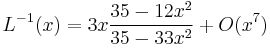
The inverse Langevin function can be approximated to within 5% accuracy by the formula^[3]

$L^{-1}(x) \approx x \frac{3-x^2}{1-x^2},$

valid on the whole interval (-1, 1). For small values of x, better approximations are the Padé approximant

$L^{-1}(x) = 3x \frac{35-12x^2}{35-33x^2} %2B O(x^7)$

and the Taylor series^[4]

$L^{-1}(x) = 3 x %2B \tfrac{9}{5} x^3 %2B \tfrac{297}{175} x^5 %2B \tfrac{1539}{875} x^7 %2B \dots$

High Temperature Limit

When $x \ll 1$ i.e. when $\mu_B B / k_B T$ is small, the expression of the magnetization can be approximated by the Curie's law:

$M = C \cdot \frac{H}{T}$

where $C = \frac{N g^2 J(J%2B1) \mu_B^2}{3k_B}$ is a constant. One can note that $g\sqrt{J(J%2B1)}$ is the effective number of Bohr magnetons.

High Field Limit

When $x\to\infty$ , the Brillouin function goes to 1. The magnetization saturates with the magnetic moments completely aligned with the applied field:

$M = N g \mu_B J$

References

^ ^a ^b ^c C. Kittel, Introduction to Solid State Physics (8th ed.), pages 303-4 ISBN 978-0471415268
^ Darby, M.I. (1967). "Tables of the Brillouin function and of the related function for the spontaneous magnetization". Brit. J. Appl. Phys. 18 (10): 1415–1417. Bibcode 1967BJAP...18.1415D. doi:10.1088/0508-3443/18/10/307
^ Cohen, A. (1991). "A Padé approximant to the inverse Langevin function". Rheologica Acta 30 (3): 270–273. doi:10.1007/BF00366640.
^ Johal, A. S.; Dunstan, D. J. (2007). "Energy functions for rubber from microscopic potentials". Journal of Applied Physics 101 (8): 084917. Bibcode 2007JAP...101h4917J. doi:10.1063/1.2723870.